Output files

After ARIADNE has finished running, it will output a series of files and plots showing the results of the fit and other information.

The most important file is the best_fit.dat which contains the best fiting parameters with the 1 sigma error bars and the 3 sigma confidence interval. Then there are pickle files for each of the used models plus a last one for the BMA, these contain raw information about the results. There is a prior.dat file that shows the priors used and a mags.dat file with the used magnitudes and filters.

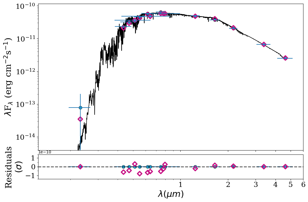
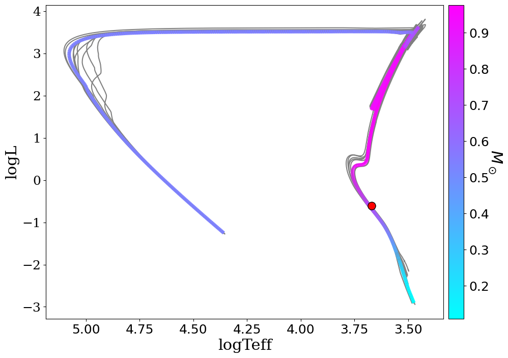
Another important output are the plots. Inside the plots folder you can find CORNER.png/pdf with the cornerplot (the plot showing the distribution of the parameters agains eachother), HR_diagram.png/pdf only for the BMA, with the HR diagram showing the position of the star, SED_no_model.png/pdf with the RAW SED showing each photometry point color coded to their respective filter (coloured by wavelength, overlaid with the blackbody fit from the photometry quality-control step, and any QC-flagged bands circled in red — see below), and SED.png/pdf with the SED with the catalog photometry plus synthetic 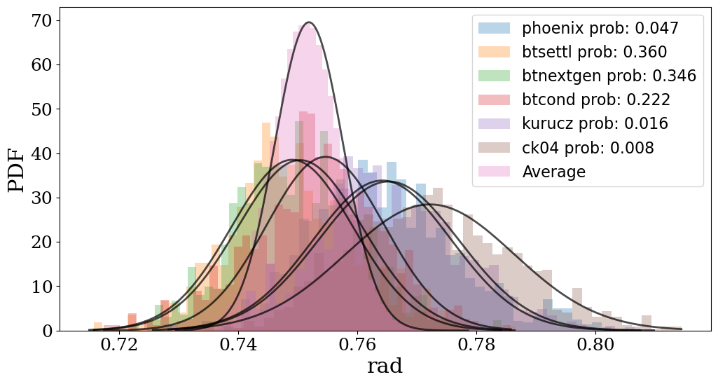photometry. If BMA was done, there’s also a histograms folder inside the plot folder with various histograms of the fitted parameters and their distribution per model, highlighting the benefits of BMA.

Examples of those figures:

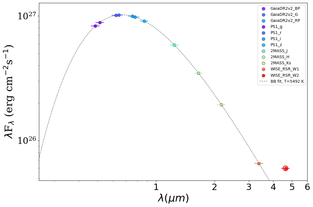
Photometry quality control

The raw SED plot doubles as a quality-control diagnostic. ARIADNE fits a blackbody to the photometry (anchored on the Gaia bands) and overlays it on SED_no_model.png. Points are coloured by effective wavelength (violet/blue at short wavelengths through to orange/red at long ones), and bands that sit more than 5σ off the fit are flagged and circled in red so you can eyeball whether a catalogue point genuinely belongs to the stellar continuum — useful for spotting blends, bad cross-matches or real infrared excesses. By default flagged bands are only warned about, not removed, so the decision stays with you.

In the example below the star is a clean ~5500 K blackbody and the WISE W2 point (circled in red) shows a clear infrared excess above the fit:

NetCDF Export (Ecosystem Interop)

As of version 1.4.0 (extended in 1.4.1), ARIADNE can export its results as an arviz DataTree in netCDF4 format. This is the canonical inter-tool format for passing full posterior distributions to downstream tools (LACHESIS, PROTEUS, etc.) without reducing to point estimates.

Exporting

After a BMA fit completes, call to_netcdf on the Fitter object:

f.fit()             # run the fit as usual
f.to_netcdf('ariadne_result.nc')

Or get the raw dictionary (useful for programmatic access without writing a file):

result = f.to_dict()
teff_samples = result['posterior']['Teff']      # shape (1, n_draws)
model_weights = result['sample_stats']['model_weights']

Reading the output

import arviz as az

dt = az.from_netcdf('ariadne_result.nc')

# BMA-weighted posterior (combined across all models)
teff = dt['posterior'].ds.Teff          # shape (chain=1, draw=100000)
print(f"Teff = {float(teff.median()):.0f} K")

# Observed photometry used in the fit
obs = dt['observed_data'].ds
print(obs.wavelength.values)            # micron
print(obs.flux.values)                  # erg/s/cm^2/micron

# Model evidence and BMA weights
cd = dt['constant_data'].ds
print(cd.model_names.values)            # e.g. ['phoenix', 'kurucz', 'btsettl']
print(cd.model_weights.values)          # e.g. [0.08, 0.26, 0.66]
print(float(cd.log_evidence))           # BMA-weighted log evidence

# Per-model posteriors (individual model fits before averaging)
phoenix = dt['posterior_phoenix'].ds
print(f"Phoenix Teff = {float(phoenix.Teff.median()):.0f} K")
print(f"Phoenix log-likelihood median = {float(phoenix.log_likelihood.median()):.2f}")

# Construct a KDE prior for downstream tools
from scipy.stats import gaussian_kde
kde = gaussian_kde(teff.values.flatten())

Since 1.4.1 you can attach the best-fit model SED before exporting, so the .nc file carries everything needed to re-plot it:

# Assuming `artist` is an SEDPlotter that has been initialized
f.out['model_sed'] = {
    'model_flux': artist.model,    # f_λ at filter wavelengths
    'wavelengths': artist.wave,
}
f.to_netcdf('ariadne_result.nc')

File structure

/
├── posterior/                          BMA-weighted combined posterior
│   ├── Teff          (chain, draw)    K
│   ├── logg          (chain, draw)    dex
│   ├── feh           (chain, draw)    dex
│   ├── radius        (chain, draw)    R_sun
│   ├── luminosity    (chain, draw)    L_sun
│   ├── distance      (chain, draw)    pc
│   ├── Av            (chain, draw)    mag
│   ├── age           (chain, draw)    Gyr          [1.4.1+, from MIST]
│   ├── iso_mass      (chain, draw)    M_sun        [1.4.1+, from MIST]
│   └── eep           (chain, draw)                 [1.4.1+, from MIST]
│
├── posterior_{model}/                  One group per stellar model used
│   ├── Teff          (chain, draw)    K
│   ├── ...
│   └── log_likelihood (chain, draw)   Per-sample log-likelihood
│
├── observed_data/                     Photometry used in the fit
│   ├── wavelength    (band,)          micron
│   ├── flux          (band,)          erg/s/cm^2/micron
│   ├── flux_err      (band,)          erg/s/cm^2/micron
│   ├── filter_names  (band,)          str           [1.4.1+]
│   ├── bandwidths    (band,)          micron         [1.4.1+]
│   └── model_flux    (band,)          erg/s/cm^2/micron  [1.4.1+, if injected]
│
├── constant_data/                     Scalar metadata
│   ├── log_evidence                   BMA-weighted log evidence
│   ├── model_weights (n_models,)      BMA posterior model probabilities
│   ├── model_names   (n_models,)      Model grid names
│   ├── best_fit_averaged__{param}     Summary stats  [1.4.1+]
│   ├── uncertainties_averaged__{param}               [1.4.1+]
│   └── confidence_interval_averaged__{param}         [1.4.1+]
│

Each model’s posterior group (e.g. posterior_phoenix, posterior_kurucz) has its own draw count reflecting the nested sampling output for that grid. The top-level posterior/ group contains the BMA-weighted resampled draws across all models, including MIST isochrone-derived parameters (age, mass, EEP) when available.

Infrared Excess

As of version 1.0, ARIADNE now allows for Infrared Excess visualization!

To visualize infrared excess you just need to add the relevant photometric observations to the Star object with the add_mag() method. After the fitting is done, you then need to initiate the Plotter object with the ir_excess parameter set to True:

artist = SEDPlotter(in_file, plots_out_folder, pdf=True, ir_excess=True)

Finally after plotting, you should get an SED figure with your manually added photometry!

Allowed filters for infrared excess plots are WISE W3, WISE W4, HERSCHEL PACS BLUE, GREEN and RED, names for these filters can be found in the filters page.